Project: Step 5.2
Statistics (Trend Curves)

Disclaimer: the automatically generated English translation is provided only for convenience and it may contain wording flaws. The original French document must be taken as reference!

Objectives: Graphically display the trend curves for certain parameters.

Complex mechanisms such as mutations are difficult to visualize over time by simply observing the contents of a culture dish. Similarly, to compare the evolution of several competing colonies, it is easier to use graphs.

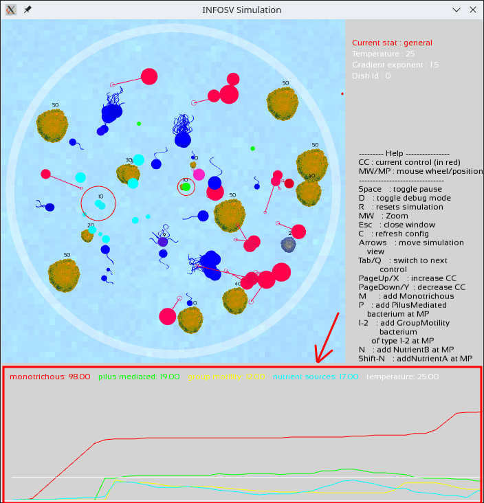
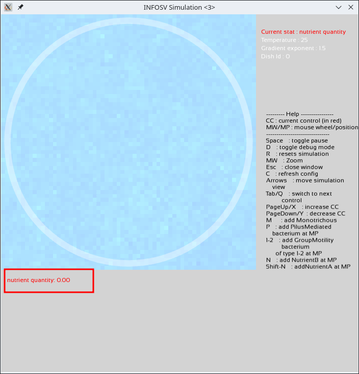
The goal of this project phase is to enable the display of trend curves for a number of parameters, according to the following model (red box):

Due to the design choices made, the statistics displayed are those of the current dish.

Understanding and extending existing code is an important programming skill. In this step, you will practice this aspect a bit more extensively than before.

To complete this step, you will need to use a variant of associative arrays (see map.pdf), namely unordered associative arrays. An unordered_map is used in a similar way to a map (the subtle differences between the two will be discussed in class shortly).

Graph class

A Graph class is provided in the archive for this step (directory src/Stats).

This class allows you to draw a set of superimposed curves. Each curve is a series of interconnected points and is associated with a title (a string of characters).

An instance of Graph is therefore a set of overlapping curves. It is characterized by a label (also a string of characters).

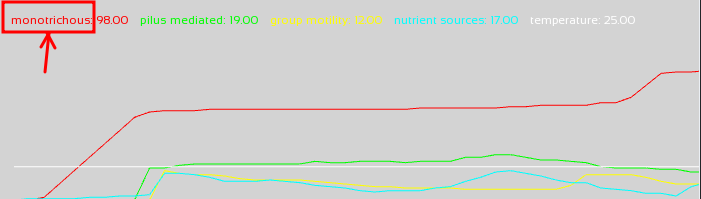
For example, above you have a graph that overlays 4 series of points:

• the one associated with the title "monotrichous" (in red) showing the evolution of the number of simple bacteria over time,
• the one associated with the title "pilus-mediated" (in green) showing the evolution of the number of pilus-bearing bacteria over time,
• etc.

In the simulation, this graph will have a label (invisible on screen) used to identify it (for example, "General" for a general statistics graph, or "nutrient quantity" for a specific graph related to nutrient quantities, etc.).

Do not confuse the label of a graph used to identify it internally with the titles associated with each of its data series ("monotrichous", in red, in the window shown in the example above):

In summary, a graph has a label and a set of point series. Each point series has a title.

The idea is to be able to display several of these Graphs and switch between them using new controls (similar to the ones you used to control the temperature and gradient exponent).

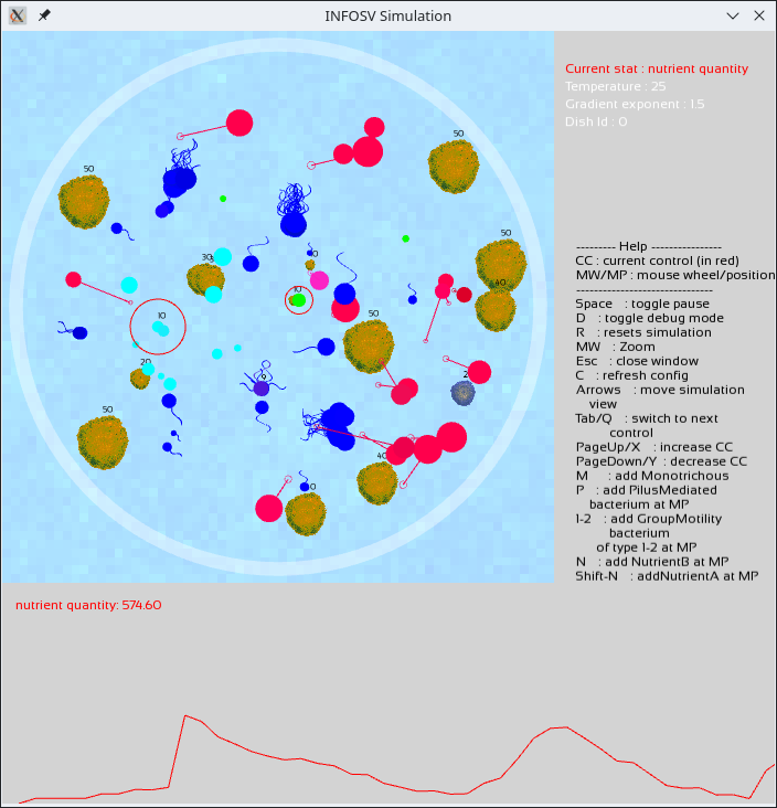
For example, when the current control (the one in red) is the statistics control, it should be possible to switch using PgUp/X to display the graph showing the total amount of available nutrients in the current dish (associated with the label nutrient quantity), this graph would, for example, only have a series of points to display (no superimposed curves):

Various constants containing strings are provided in the file Utility/Constants.hpp. In particular, you will find the constant s::GENERAL for the label "General".

At this stage, you are asked to complete the Stats class (see below) to manage all the graphs you wish to display as part of this simulation and to add the functionality to switch from one graph to another.

The Stats class will therefore allow you to display multiple graphs, each graph being associated with a label that describes it.

The Application class now contains an attribute of type Stats* and offers a number of features related to this attribute. It also performs operations on this attribute (such as calling its drawOn method).

It is the graphical programs, such as the class FinalApplication, which, by calling the method addGraph inherited from Application, will define:

• the label associated with a graph;
• the set of point series that are associated (designated by their title);
• as well as the lower and upper bounds of the value ranges associated with these point series.

It is the FinalApplication class that, through calls to the addGraph method inherited from Application, will define the label associated with a graph, the set of point series associated with it (designated by their titles), as well as the lower and upper bounds of the value ranges associated with these point series.

Take a look at lines 25 and 26 of the onRun method in FinalApplication.cpp (currently commented out). These lines are specifically responsible for adding graphs to this program.

The Stats class

An object of the Stats class is essentially characterized by a set of graphs (a set of std::unique_ptr<Graph>) and a set of labels associated with these graphs (strings). This is a drawable object that evolves over time.

Each graph (and therefore each label as well) will be associated with an integer identifier. For example, identifier zero will be associated with the graph labeled "general," identifier 1 will be associated with the graph labeled "nutrient quantity," and so on.

An object of type Stats will also be characterized by the active identifier (the one corresponding to the option selected in the controls): the drawing method of Stats will draw only the graph with the active identifier.

In the Stats class you will complete:

• the method void setActive(int id) allowing the value id to be assigned to the active identifier;
• the method std::string getCurrentTitle() which returns the label of the current graph (the one corresponding to the active identifier);
• the method next() which increments the active identifier (modulo the number of graphs: it wraps around to zero if the active identifier is that of the last possible graph);
• and the method previous() allowing the active identifier to be decremented (it wraps around to the value of the last possible graph if the active identifier becomes less than zero).

[Question Q5.3]: Which data structure(s) do you choose for the set of graphs and the set of titles in the Stats class? Answer this question in your REPONSES file and make the corresponding additions to your code.

You will also complete, in the Stats class:

• The method reset that clears all point series from the graphs and restarts the display from the origin (in fact, the graphs store the point series to be drawn and connected, and this method clears those series).
  Examine the code for the Graph class to see which method to call.
• The method addGraph that allows you to add a graph to the collection of graphs.
  This method is used by the method of the same name in the Application class: the parameters are, in order: the graph’s identifier (an int), its title (which is also the tab’s title and is a string), the set of curve titles for the graph (a vector of string), the minimum and maximum values (min and max) between which the curve points are displayed (of type double), and a Vec2d (named size) specifying the dimensions of the graphics window in which the display occurs. The method prototype is then given as follows:

  void addGraph(
    int id,
    const std::string &title,
    const std::vector<std::string> &series,
    double min,
    double max,
    const Vec2d &size
  );
  

• Reset the pointer to the Graph associated with the parameter ID by associating it with a new Graph, dynamically allocated (using the reset method of unique_ptr).
The following example shows how to use this method:

  #include <iostream>
  #include <memory>

  int main() {
    std::unique_ptr<int> p(new int(1));
    std::cout << *p << std::endl; // 1
    p.reset(new int(2));
    std::cout << *p << std::endl; // 2
    return 0;
  }

• Update the title of the graph associated with the identifier, using the title passed as a parameter.
• Ensure that the ID passed as a parameter is listed as the active ID.

    getApp().resetStats(); // call to the Stats::reset method
  

Test 18: Preparing to display the curves

To test this section, you can continue using the final application provided in src/Tests/GraphicalTests/FinalApplication.cpp, which can be launched using the application target. Be sure to first uncomment the addition of the graphs (lines 25 and 26 of FinalApplication) and change the parameter on line 23 from false to true (to enable the display of statistics).

Note that the size of the graph area used to display statistics can be configured in the file app.json:

    "window":{
        "antialiasing level":4,
        "title":"INFOSV Simulation",
        "simulation":{
            "width":700,
            "height":700
        },
        "stats":{
            "width":200 // For example, replace 200 with 300 here
        },
        "control":{
            "width":300
        }
  

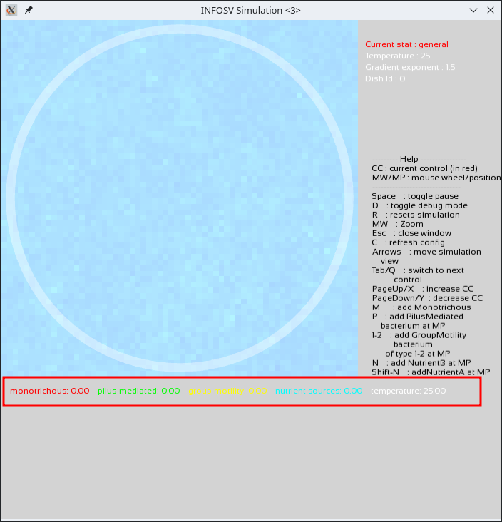
You should then simply see the labels associated with the upcoming curves displayed (without the actual curves being shown at this point). For example, for the graph labeled "general" :

Graph Data

To actually display curves, you must populate the data series associated with each graph. This is what you are asked to do in the following.

The Stats::update method

The data is not updated with every update but every sf::seconds(getAppConfig()["stats"]["refresh rate"].toDouble()); seconds.

The algorithm for updating the data is then as follows.

For each graph:

1. calculate the new data to be inserted into each series of the graph;
2. insert each new data point into its series;

Let’s start with an example. Suppose we are updating the Graph "general" (as described above). It consists of 5 series of points: one for the number of single-tentacled bacteria, another for the number of multi-tentacled bacteria, and so on. These series can be schematized as follows:

{ "monotrichous", {p11, p12, ...  p1j}}
{"pilus mediated", {p21, p22, ...  p2j}}
{"group motility", {p31, p32, ...  p3j}}
{"nutrient sources", {p41, p42, ...  p4j}}
{"temperature", {p51, p52, ...  p5j}}

Step 1 of the algorithm above must therefore calculate the set

{new_data = { "simple bacteria", p1j+1}, {"twitching bacteria", p2j+1}, ... {"nutrient sources", p4j+1}...}

Step 2 of the algorithm “injects” this data into the graph to update the series:

{ "monotrichous", {p11, p12, ...  p1j+1}}
{"pilus mediated", {p21, p22, ...  p2j+1}}
{"group motility", {p31, p32, ...  p3j+1}}
{"nutrient sources", {p41, p42, ...  p4j+1}}
{"temperature", {p51, p52, ...  p5j+1}}

Step 2 of the algorithm can be implemented very simply by calling Graph::updateData(deltaT, new_data) on the graph to be updated, where deltaT is the time elapsed since the last data update and new_data is the set of new data for each series (as described in the previous example).

You are therefore asked to implement a method std::unordered_map<std::string, double> Lab::fetchData(const std::string &) that takes the graph title (a string) as a parameter and returns the corresponding new_data set (also consider whether this method should be marked as const or not).

For example:

• If the graph title is the value of s::GENERAL, then fetchData will return an unordered_map structured by the new_data from the example above.
• If the title is s::NUTRIMENT_QUANTITY, the contents of new_data will be calculated in a similar manner.

[Question Q5.4] Which methods do you plan to add or modify, and in which classes, to perform the desired counts and construct the new_data sets? In other words, how can you count the number of instances of a certain class? Answer this question in your REPONSES file and implement the necessary code.

Test 19: Displaying Population Growth Curves

Run your simulation as before and create different types of bacteria. You should see the growth curves for the populations and the amount of nutrients displayed. Suddenly create a large number of bacteria of a certain type, and you should be able to see that the growth curve "reacts" accordingly. Verify that you can switch between statistics using the provided control keys:

Verify that the statistical curves reset properly when switching between culture dishes.

Test 20: Adding new curves (bonus)

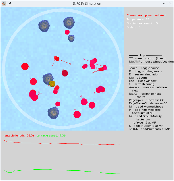
Finally, complete the curve display by enabling the visualization of trend curves for variable numerical parameters. For example, for bacteria with tentacles, the average lengths and speeds of the tentacles.

Run your simulation as before. You should be able to visualize the evolution of the numeric parameters of your bacteria; here is an example for bacteria with tentacles:

You now have a complete simulation tool. Try configuring it to find conditions that, for example, allow for fluctuations in the numbers of the various populations without causing the extinction of any of them.